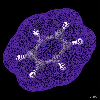
Click on a link below to see what it does. You can also type a command in the box below the model to see its effect. The script run in this case was ch3cl_map.jvxl; set perspectivedepth off;moveto 1 345 456 567 49;set scriptQueue on;set loglevel 4.
This page can be used to experiment with the 10.x prototype. Files are available in this directory. Comments? Suggestions? Bob Hanson
Jmol 11.5.46 adds functionXY as a mapping source.That is, you can take any object such as a surface, a sphere, a plane, another function -- anything -- and map it with color based on a function f(x,y). See isosurface.htm.A negative value for the number of x values indicates that the function should return a string containing the Z values.
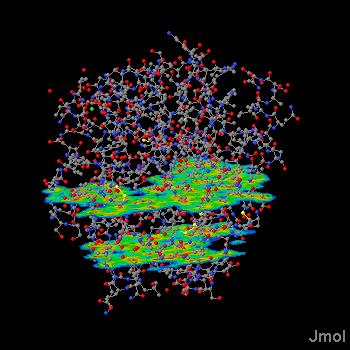
28. slices through a molecular surface and new way to define plane
Jmol uses a unique algorithm to calculate surfaces. Each position in space is given a value that is its distance from the nearest surface point. What this means is that a "surface" is really an "isosurface with cutoff 0". And what that means is that a surface is no different in terms of visualization from a molecular orbital or other atom-based spacial property. Jmol 10.9.71 allows you to generate slices through a surface.
generated from the following command (which takes several seconds on my machine). Note the new way to define a plane simply in terms of three points -- (atom)s or {coordinate}s
27. isosurface hkl -- planar slices using Miller indices
Jmol 10.9.72 introduces the "hkl" keyword indicates that the next three numbers in braces are Miller indices. Note that all coordinates are implicitly fractional. A faster alternative is to use "solvent 0" instead of "molecular".
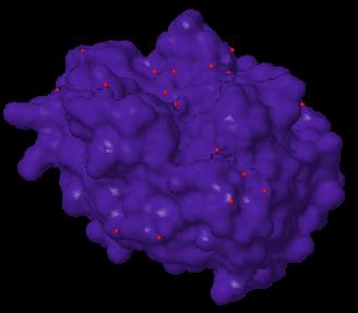
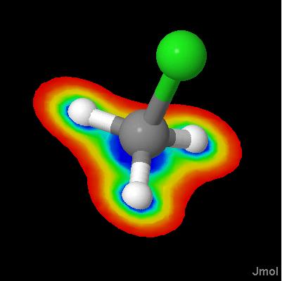
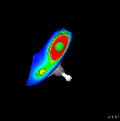
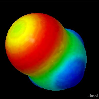
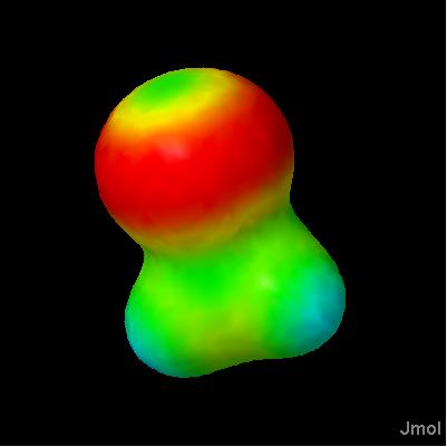
Jmol 10.9.63 introduces isosurface MEP, with which you can display molecular electrostatic potentials. These potentials are calculated from partial charge data present in a file; Jmol cannot calculate these charges. Just the MEP:
NOTE -- in testing 10.x.19 and writing up documentation I have changed some of the isosurface parameters. Namely, "fileindex n" is gone. One simply indicates the surface number after the quoted filename similarly to the way you can indicate a model number after a quoted filename in a "load" command. In addition, I have simplified the command syntax by allowing ALL construction/color parameters up front. See the documentation
Jmol 10.x.09 introduces VERY compact orbitals and other molecular properties as isosurfaces. These files are generated by Jmol from Gaussian CUBE files with compression ratios on the order of 400 to 600:1. This is possible because JVXL files do not allow for variable cutoffs. check out the new "Jmol Voxel File" format at ch3cl.jvxl. For a discussion see JVXL-format.pdf. Many examples follow.
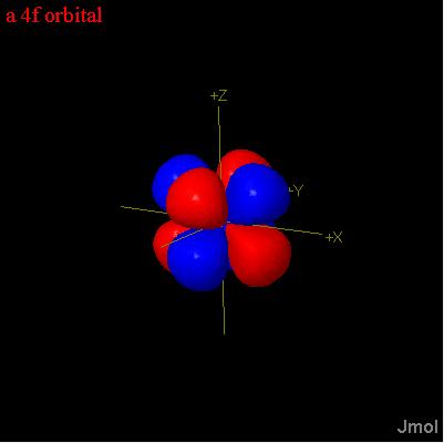
23. hydrogen-like orbitals calculated using the Schroedinger equation
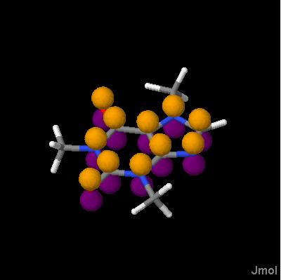
orbitals are defined by three required quantum numbers (n, l, m) and two additional optional numbers: Zeff(effective nuclear charge, default 6), and an optional resolution in the form of a number of points per angstrom (default 10). In addition, you can specify a cutoff
You can center a hydrogen-like orbital at any position in molecular space using {x y z} or at any atom using an atom expression. Required parameters include the three quantum numbers: n, l, and m.
You can center an orbital just like a lobe -- on a given point in space, on an atom, or on the geometrical center of a group of atoms in an atom expression.
You can distort a hydrogen-like orbital using the ANISOTROPY keyword followed by a coordinate indicating the distortion along each of the three axes. "Look, Ma! A yo-yo!"
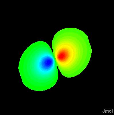
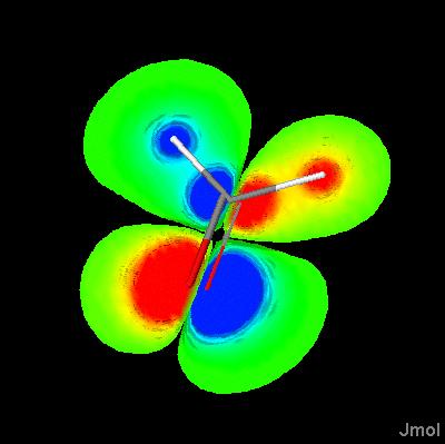
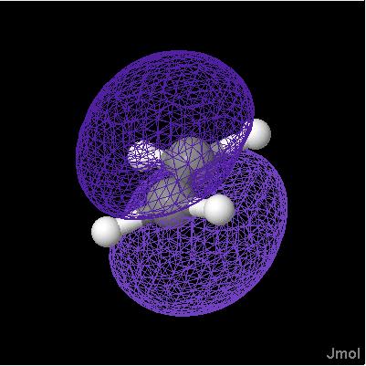
orbitals are generally depicted as dichromatically colored isosurfaces. The surface itself is based on the square of the wave function, psi (so that it represents probability); the color is based on the sign of psi. Effectively, one isosurface (sign of psi) is being used to map color onto another isosurface (psi squared).
Notice the problem there -- orbitals should be only two colors, not a mix. So we add the keyword "sign" to indicate we want the coloring based on the SIGN of the value in the second CUBE file, not the actual value itself. Note that dxy-phase.cube is a very small, simple file.
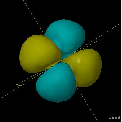
In addition, to simpify matters with the eight "standard" p/d orbitals, you can simply define the phase of the coloring as one of the following: x, y, z, xy, xz, yz, x2-y2, or z2. Here we are using a set of d orbitals in one convenient 10Kb file: (a compression ratio of 468:1)
Jmol 10.x.25 includes a new command that allows quick scanning through molecular orbitals almost like they were frames. The MO command takes several simple forms. See mo.htm
20. direct calculation of molecular orbitals (no cube files)
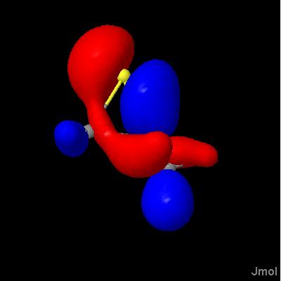
Jmol 10.x.20 can render many standard calculated molecular orbitals WITHOUT cube files. Current readers include GAUSSIAN (keywords pop=full gfprint) and GAMESS output files, and SMOL, SPARCHIVE, and WebMO data files. Most ab initio (STO-3G, 3-21G*, 6-31++G**, etc.) and semi-empirical (AM1, PM3) basis sets can be rendered. The MO command is simpler to use, but less flexible. a WebMO file:
The isosurface command can be used to manipulate the phased sections of the MO independently. The key is to indicate the cutoff with an explicit "+" or "-" sign.
You can retrieve the data used for these calculations using getProperty "auxiliaryInfo", which returns JavaScript Object Notation (JSON), which is being translated into JavaScript array notation here. Gaussian output: The second frame holds the information we want
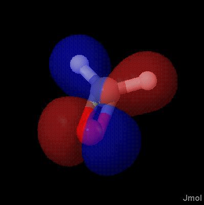
SMOL RHF/3-21G calc on XeF4 from http://introchem.chem.okstate.edu/jmol/molecules/. I have removed the unnecessary encoded isosurface data (1.0MB --> 147KB), so this is no longer a true SMOL file. This file contains 75 molecular orbitals.
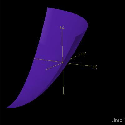
Jmol 10.x.16 introduces cartoonish "lobes" that can be placed anywhere. They form the basis for hybrid orbitals and cartoon-like LCAO orbitals. The shape used is the central section of the 3dz2 orbital.
The four numbers in brackets describe the orientation and "eccentricity" of the lobe. The first three numbers describe the vector axis of the lobe. The fourth number is the lateral distortion of the lobe relative to a hydrogen 3dz2 orbital lobe.
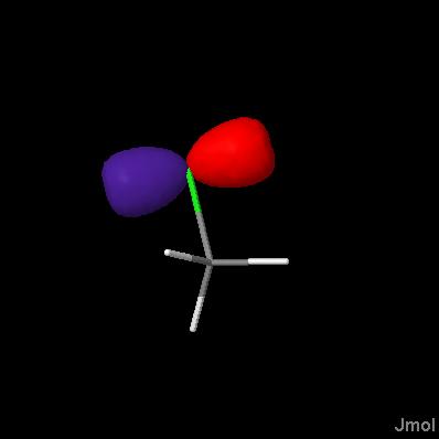
Jmol 10.x.17 introduces tear-drop shaped "cartoon" orbitals that can be used to depict the atomic orbitals generally discussed in relation to the linear combination of atomic orbitals (LCAO) approximation, Hueckel theory, and hybridization. The lobes use a distortion of 0.7 relative to a standard 3dz2 orbital.
p-orbital and in-plane hybrid for an sp2-hybridized atom: the default orientation for the positive end of the z orbital is toward positive z in the molecular frame.
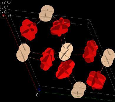
the four parameters are the "eccentricity" of the ellipse -- the x,y,z coordinates of the vector defining the "c" axis followed by the a/c = b/c ratio of the two perpendicular axes. Future plans are to support Ortep anisotropies, which allow all three axes to be independently scalable, but that has not been implemented yet.
Planes of electrostatic potential are particularly suitable to the JVXL format, because they do not require any surface or edge fraction data. Originally my thought was that all that is needed was to compress the color data. plane.jvxl is only 952 bytes!
But if you look closely, you will see the problem. The rendition is very blocky. This is because we are not interpolating enough. Here we use the actual cube file, so we can select a plane. The plane definition takes the form of four numbers, {a b c d} where ax + by + cz + d = 0. The three numbers also define the vector representing the normal to the plane. Math World: plane. Go ahead and try different planes. Just change the numbers in the textbox below the applet and press the [ENTER] key.
You can specify the number of contours you want to use. The default is 11. Setting this value to 1 allows a comparison to no Marching Squares. A negative number indicates that you want to only see one single contour.
for orbital slices it is important to specify an odd number of contours. (The default number of contours is 11 for this reason.) Compare the following two scripts. Notice that when the contours is even, the two lobes are oddly different. This is because one contour is right a 0.00, and that leads to a contour that is too sensitive to random noise in the sampling method.
You can now use user-defined functions to create a surface, and you can map cube data onto an arbitrarily defined function(x,y). If you wish, you can then "show isosurface" and put the surface into a JVXL file for delivery over the web. In this case we are calling the JavaScript function curveXY(), which evaluates to get the actual function value. The x and y coordinates passed to this function are NOT the actual x and y coordinates of the point. They are the x and y coordinates of the point in the "voxel cube" defined by the origin and three vector definitions listed after the function name in the command. Each vector definition includes the number of voxels along that direction and the xyz coordinates defining the grid size in that direction. These vectors can be in any direction, but they should be perpendicular if the surface is to be color-mapped. Units are Angstroms. A negative value for the number of x values indicates that the function should return a string containing the Z values. A negative number for both X and Y indicate that the function expects a float[][] array in the fourth parameter and will fill that directly. (Go ahead and change that function, click here to "set" the function, and then see what happens when you click the link below again.)
12. solvent examples -- using select and resolution
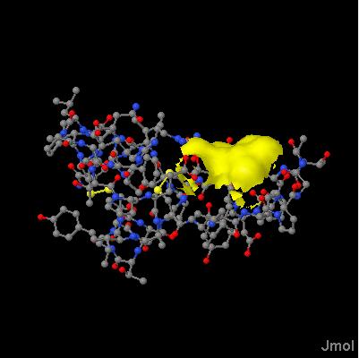
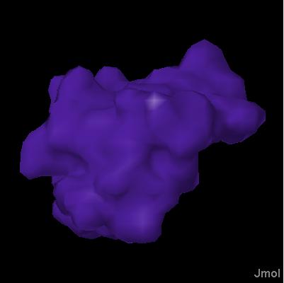
starting with Jmol 10.x.23, selecting only a subset of the atoms displays only the corresponding subset of the overall surface. Note that we use the script file groups.scr here for quick reference to specific organic groups.
It may take several seconds to create a solvent surface, but the JVXL file option provides a way of doing this calculation once, then just delivering the data to users.
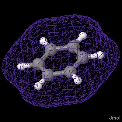
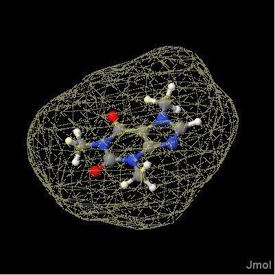
A solvent-accessible surface is the surface described the CENTER of a spherical idealized solvent of a specified radius rolling around the molecule. Jmol 10.x.18 can display this surface using the SASURFACE keyword:
Can you tell the difference? (They are ever so slightly different.) Next is ethene, compressed 416:1 relative to ethene-HOMO.cub and 65:1 relative to ethene-HOMO.cub.gz
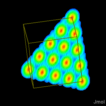
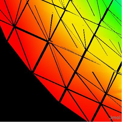
The key turns out to be an adaptation of the 3D "Marching Cubes" data interpolation algorithm to two dimensions -- "Marching Squares". For the JVXL equivalent, we opt for a higher level of precision in the data compression. The files are larger than before, but still afford 400-500:1 compression ratios.
What you are looking at is a set of 10 contours that have then been triangulated using the Marching Square algorithm with linear shading through each triangle. Here is a closeup:
When the surface is a plane, our eyes are particularly sensitive to differences in shading and color. JVXL files are not quite the same as CUBE files, and this is noticeable for slices. Still, the effect is subtle, because it is only slight variations in the square-contour intersection points that we are seeing. CUBE file (593K gzipped)
JVXL files can be combined into one file with multiple surfaces. You can just do this by hand. Make sure that the FIRST number on the JVXL dataset definition line is a negative number indicating how many isosurfaces are contained in the file. (This particular file uses older data that is not treated with Marching Squares, so it is somewhat blocky.)
5. isosurface FIXED/MODELBASED and multiple models
As in the case of draw objects (points, lines, planes) there may be times when isosurfaces are intended to be displayed for all models ("FIXED") and times when they are model-based. The default assumption is MODELBASED, but one can also specify FIXED. Note that we use the 1001, 2001, 3001,... notation for frames because they come from different files (or so the applet thinks!). Using this technique you can select which orbitals to view based on which frames are currently visible.
Most CUBE/JVXL files have file coordinates in them, but you do not need to use those coordinates. You can instead load one file and then apply the isosurface from another. Just making the point here:
2. appendix: testing the idea of vertex normal grouping
Along the way, I noticed that the specular refection was not optimal. The problem turned out to be a problem with the "average normals" used at the vertices of the triangles. The problem is now fixed.see jvxl-compare-normal.jpg and jvxl-compare-normal2.jpg.
Miguel Howard wrote the original isosurface code using the Marching Cube algorithm. I used that as a basis to adapt the Marching Squares algorithm, which was kindly suggested to me by Olaf Hall-Holt. Fast gaussian molecular orbital calculations are based on algorithms by Daniel Severance and Bill Jorgensen. I thank Won Kyu Park for pointing me to this work. The JVXL file format was my own idea.